defrender_rectangle(rectangle_vertices, focal, principal_point, image_dimensions): """Renders a rectangle on the image plane. Args: rectangle_vertices: the four 3D corners of a rectangle. focal: the focal lengths of a projective camera. principal_point: the position of the principal point on the image plane. image_dimensions: the dimensions (in pixels) of the image. Returns: A 2d image of the 3D rectangle. """ image = np.zeros((int(image_dimensions[0]), int(image_dimensions[1]), 3))#初始化一张全空白图像(w,h,[r,g,b]) vertices_2d = perspective.project(rectangle_vertices, focal, principal_point) vertices_2d_np = vertices_2d.numpy() top_left_corner = np.maximum(vertices_2d_np[0, :], (0, 0)).astype(int) bottom_right_corner = np.minimum( vertices_2d_np[1, :], (image_dimensions[1] - 1, image_dimensions[0] - 1)).astype(int) for x inrange(top_left_corner[0], bottom_right_corner[0] + 1): for y inrange(top_left_corner[1], bottom_right_corner[1] + 1): c1 = float(bottom_right_corner[0] + 1 - x) / float(bottom_right_corner[0] + 1 - top_left_corner[0]) c2 = float(bottom_right_corner[1] + 1 - y) / float(bottom_right_corner[1] + 1 - top_left_corner[1]) image[y, x] = (c1, c2, 1) return image
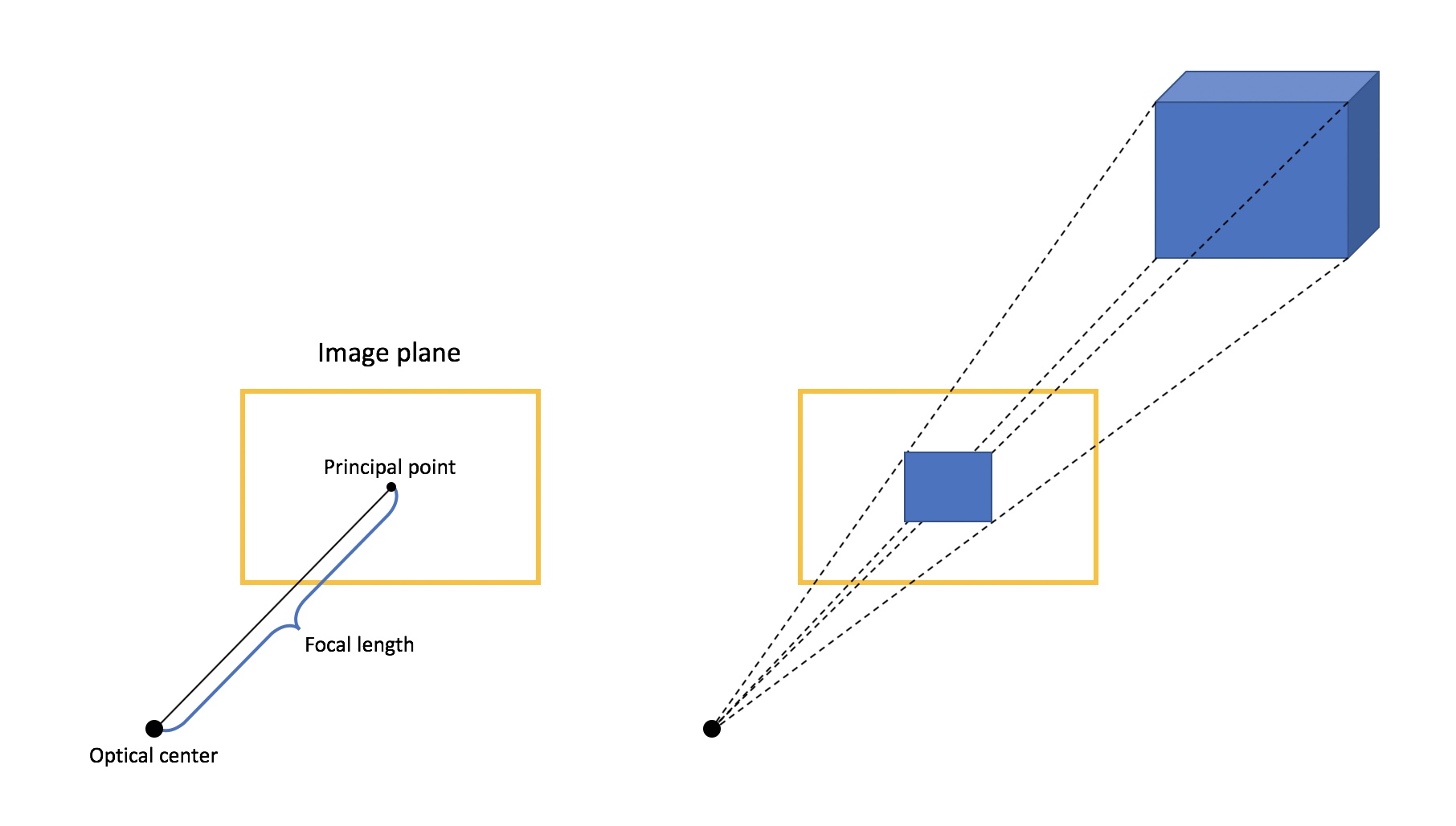
# Sets up the vertices of the rectangle.
rectangle_depth = 1000.0
rectangle_vertices = np.array(
    ((-150.0, -75.0, rectangle_depth), (150.0, 75.0, rectangle_depth)))

# Sets up the size of the image plane.
image_width = 400
image_height = 300
image_dimensions = np.array((image_height, image_width), dtype=np.float64)

# Sets the horizontal and vertical focal length to be the same. The focal length
# picked yields a field of view around 50degrees.
focal_lengths = np.array((image_height, image_height), dtype=np.float64)
# Sets the principal point at the image center.
ideal_principal_point = np.array(
    (image_width, image_height), dtype=np.float64) / 2.0

# Let's see what our scene looks like using the intrinsic paramters defined above.
render = render_rectangle(rectangle_vertices, focal_lengths, ideal_principal_point,
                          image_dimensions)
_ = plt.imshow(render)
## 输出误差 defprint_errors(focal_error, center_error): print("Error focal length %f" % (focal_error,)) print("Err principal point %f" % (center_error,))
Let’s now define the values of the intrinsic parameters we are looking for, and an initial guess of the values of these parameters.
1 2 3 4 5 6 7 8 9 10 11 12 13 14
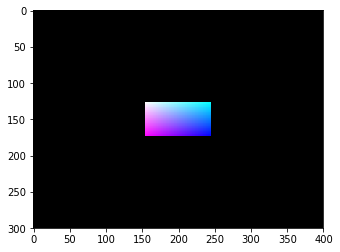
defbuild_parameters(): # Constructs the intrinsic parameters we wish to recover. real_focal_lengths = focal_lengths * np.random.uniform(0.8, 1.2, size=(2,)) real_principal_point = ideal_principal_point + (np.random.random(2) - 0.5) * image_width / 5.0
# Initializes the first estimate of the intrinsic parameters. estimate_focal_lengths = tf.Variable(real_focal_lengths + (np.random.random(2) - 0.5) * image_width) estimate_principal_point = tf.Variable(real_principal_point + (np.random.random(2) - 0.5) * image_width / 4) return real_focal_lengths, real_principal_point, estimate_focal_lengths, estimate_principal_point
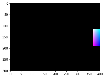
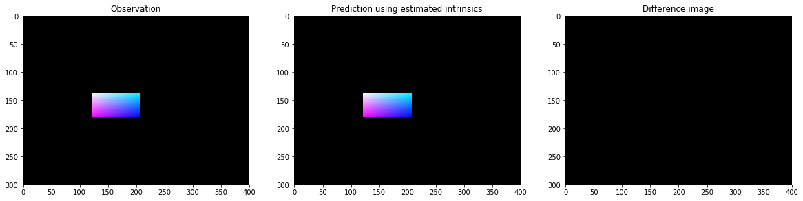
As described earlier, one can compare how the 3D object would look using the current estimate of the intrinsic parameters, can compare that to the actual observation. The following function captures a distance beween these two images which we will seek to minimize.
All the pieces are now in place to solve the problem; let’s give it a go!
Note: the residuals are minimized using Levenberg-Marquardt, which is particularly indicated for this problem. First order optimizers (e.g. Adam or gradient descent) could also be used.